Molecular dynamics application example
Go to:
The C-type lectin receptor langerin
Notebook configuration
[1]:
import sys

import matplotlib.pyplot as plt
import matplotlib as mpl
import numpy as np
import sklearn
from sklearn.neighbors import KDTree
from sklearn.metrics import pairwise_distances
from tqdm.notebook import tqdm

import commonnn
from commonnn import cluster, plot, recipes, _types, _fit, _bundle
Print Python and package version information:
[2]:
# Version information
print("Python: ", *sys.version.split("\n"))

print("Packages:")
for package in [mpl, np, sklearn, commonnn]:
    print(f"    {package.__name__}: {package.__version__}")
Python:  3.9.0 | packaged by conda-forge | (default, Nov 26 2020, 07:57:39)  [GCC 9.3.0]
Packages:
    matplotlib: 3.9.4
    numpy: 1.26.4
    sklearn: 1.6.1
    commonnn: 0.0.4
We use Matplotlib to create plots. The matplotlibrc file in the root directory of the CommonNNClustering repository is used to customize the appearance of the plots.
[3]:
# Matplotlib configuration
mpl.rc_file(
    "../../matplotlibrc",
    use_default_template=False
)
[4]:
# Axis property defaults for the plots
ax_props = {
    "xlabel": None,
    "ylabel": None,
    "xticks": (),
    "yticks": (),
    "aspect": "equal"
}
Helper functions
[5]:
def draw_evaluate(clustering, axis_labels=False, plot_style="dots"):

    fig, Ax = plt.subplots(
        1, 3,
        figsize=(
            mpl.rcParams['figure.figsize'][0],
            mpl.rcParams['figure.figsize'][1] * 0.5)
        )

    for dim in range(3):
        dim_ = (dim * 2, dim * 2 + 1)

        ax_props_ = {**ax_props}
        if axis_labels:
            ax_props_.update(
                {"xlabel": dim_[0] + 1, "ylabel": dim_[1] + 1}
            )

        _ = clustering.evaluate(
            ax=Ax[dim],
            plot_style=plot_style,
            ax_props=ax_props_,
            dim=dim_
            )

        Ax[dim].yaxis.get_label().set_rotation(0)
The C-type lectin receptor langerin
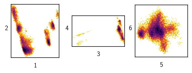
Let’s read in some “real world” data for this example. We will work with a 6D projection from a classical MD trajectory of the C-type lectin receptor langerin that was generated by the dimension reduction procedure TICA.
[6]:
langerin = cluster.Clustering(
    np.load("md_example/langerin_projection.npy", allow_pickle=True),
    alias="C-type lectin langerin"
    )
After creating a Clustering instance, we can print out basic information about the data. The projection comes in 116 parts of individual independent simulations. In total we have about 26,000 data points in this set representing 26 microseconds of simulation time at a sampling timestep of 1 nanoseconds.
[57]:
print(langerin.root.info())
alias: 'root'
hierarchy_level: 0
access: components
points: 26528
children: 0
[58]:
print(langerin.root._input_data.meta)
{'access_components': True, 'edges': [56, 42, 209, 1000, 142, 251, 251, 251, 251, 251, 251, 251, 221, 221, 221, 221, 221, 221, 221, 221, 221, 221, 221, 221, 221, 221, 221, 221, 221, 221, 221, 221, 221, 221, 221, 221, 221, 221, 221, 221, 221, 221, 221, 221, 221, 221, 221, 221, 221, 221, 221, 221, 221, 221, 221, 221, 221, 221, 221, 221, 221, 221, 221, 144, 636, 221, 221, 221, 221, 221, 221, 221, 221, 221, 221, 221, 221, 221, 221, 221, 221, 221, 221, 221, 221, 221, 221, 221, 221, 221, 221, 221, 221, 221, 221, 221, 221, 221, 221, 221, 221, 221, 221, 221, 221, 221, 221, 221, 221, 221, 221, 221, 221, 221, 221, 221]}
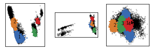
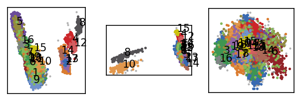
Dealing with six data dimensions we can still visualise the data quite well.
[59]:
draw_evaluate(langerin, axis_labels=True, plot_style="contourf")
After a few preliminary checks, we will partition that data by 1-step threshold-based clustering and then also by using a semi-automatic and an automatic hierarchical clustering approach for comparison.
Preliminary checks
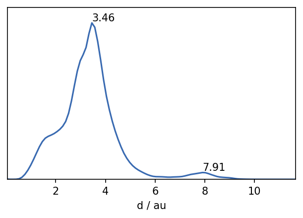
So let’s begin. A quick look on the distribution of distances in the set gives us a first feeling for what might be a suitable value for the neighbour search radius r.
[60]:
# Keep only upper triangle of the distance matrix to deduplicate
distances = pairwise_distances(
    langerin.input_data
)[np.triu_indices(langerin.root._input_data.n_points)].flatten().astype(np.float32)

fig, ax = plt.subplots()
_ = plot.plot_histogram(ax, distances, maxima=True, maxima_props={"order": 5})
[61]:
# Free memory
%xdel distances
We can suspect that values of r of roughly 2 or lower should be a good starting point. The maximum in the distribution closest to 0 defines a reasonable value range for \(r\). We can also get a feeling for what values \(n_\mathrm{c}\) could take on by checking the number of neighbours each point has for a given search radius.
[62]:
# Can take a couple of minutes...
min_n = []
max_n = []
mean_n = []


tree = KDTree(langerin.input_data)
r_list = np.arange(0.25, 3.25, 0.25)
for r in tqdm(r_list):
    n_neighbours = [
        x.shape[0]
        for x in tree.query_radius(
            langerin.input_data, r, return_distance=False
        )
    ]

    if r == 2.0:
        n_neighbours_highlight = np.copy(n_neighbours)

    min_n.append(np.min(n_neighbours))
    max_n.append(np.max(n_neighbours))
    mean_n.append(np.mean(n_neighbours))
---------------------------------------------------------------------------
KeyboardInterrupt                         Traceback (most recent call last)
Cell In[62], line 12
      8 r_list = np.arange(0.25, 3.25, 0.25)
      9 for r in tqdm(r_list):
     10     n_neighbours = [
     11         x.shape[0]
---> 12         for x in tree.query_radius(
     13             langerin.input_data, r, return_distance=False
     14         )
     15     ]
     17     if r == 2.0:
     18         n_neighbours_highlight = np.copy(n_neighbours)

KeyboardInterrupt:
[ ]:
h, e = np.histogram(n_neighbours_highlight, bins=50, density=True)
e = (e[:-1] + e[1:]) / 2

fig, ax = plt.subplots()
# ax.plot([2.0, 2.0], (e[0], e[-1]), "k")
ax.fill_betweenx(
    e, np.full_like(e, 2.0), 2.0 + h * 1000,
    edgecolor="k", facecolor="gray"
)
min_line, = ax.plot(r_list, min_n, "k")
max_line, = ax.plot(r_list, max_n, "k")
mean_line, = ax.plot(r_list, mean_n)

ax.legend(
    [min_line, mean_line], ["min/max", "mean"],
    fancybox=False, framealpha=1, edgecolor="k"
)

ax.set(**{
    "xlim": (r_list[0], r_list[-1]),
    "xlabel": "$r$",
    "ylabel": "#neighbours",
})
[(0.25, 3.0), Text(0.5, 0, '$r$'), Text(0, 0.5, '#neighbours')]
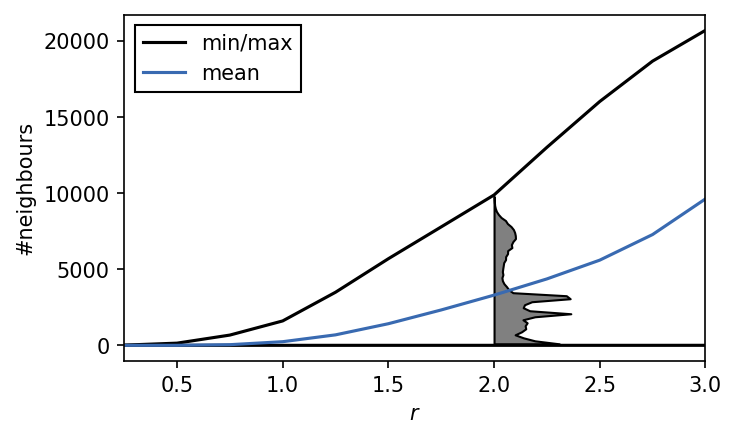
In the radius value regime of 2 and higher the number of neighbours per point quickly approaches the number of points in the whole data set. We can interpret these plots as upper bounds (max: hard bound; mean: soft bound) for \(n_\mathrm{c}\) if \(r\) varies. Values of \(n_\mathrm{c}\) much larger than say 5000 probably wont make to much sense for radii below around 2.0. If the radius cutoff is set to \(r=1\), \(n_\mathrm{c}\) is already capped at a few hundreds. We can also see that for a radius of 2.0, a substantial amount of the data points have only very few neighbours. Care has to be taken that we do not loose an interesting portion of the feature space here when this radius is used.
Clustering root data
Let’s attempt a first clustering step with a relatively low density criterion (large r cutoff, low number of common neighbours \(n_\mathrm{c}\)). When we cluster, we can judge the outcome by how many clusters we obtain and how many points end up as being classified as noise. For the first clustering steps, it can be a good idea to start with a low density cutoff and then increase it gradually (preferably by keeping \(r\) constant and increasing \(n_\mathrm{c}\)). As we choose higher density criteria the number of resulting clusters will rise and so will the noise level. We need to find the point where we yield a large number of (reasonably sized) clusters without loosing relevant information in the noise regions. Keep in mind that the ideal number of clusters and noise ratio are not definable and highly dependent on the nature of the data and your (subjective) expectation if there is no dedicated way of clustering validation.
[ ]:
# Use a fast clustering recipe here
r = 1.5
neighbourhoods, sort_order, revert_order = recipes.sorted_neighbourhoods_from_coordinates(langerin.input_data, r=r, sort_by="both")
langerin_neighbourhoods = cluster.Clustering(
    neighbourhoods, recipe="sorted_neighbourhoods"
)
[ ]:
langerin_neighbourhoods.fit(radius_cutoff=r, similarity_cutoff=2, member_cutoff=10)
langerin.labels = langerin_neighbourhoods.labels[revert_order]
-----------------------------------------------------------------------------------------------
#points   r         nc        min       max       #clusters %largest  %noise    time
26528     1.500     2         10        None      11        0.702     0.005     00:00:0.311
-----------------------------------------------------------------------------------------------
[ ]:
draw_evaluate(langerin)
We obtain a low number of noise points and a handful of clusters so we are at least not completely of track here with our initial guess on \(r\). To get a better feeling for how the clustering changes with higher density-thresholds, one could scan a few more parameter combinations.
[ ]:
for c in tqdm(np.arange(0, 105, 1)):
    langerin_neighbourhoods.fit(radius_cutoff=r, similarity_cutoff=c, member_cutoff=10, v=False)
langerin.root._summary = langerin_neighbourhoods.root._summary
[ ]:
df = langerin.summary.to_DataFrame()
df[:10]
| n_points | radius_cutoff | similarity_cutoff | member_cutoff | max_clusters | n_clusters | ratio_largest | ratio_noise | execution_time | |
|---|---|---|---|---|---|---|---|---|---|
| 0 | 26528 | 1.5 | 2 | 10 | <NA> | 11 | 0.702201 | 0.005428 | 0.482993 |
| 1 | 26528 | 1.5 | 2 | 10 | <NA> | 11 | 0.702201 | 0.005428 | 0.442934 |
| 2 | 26528 | 1.5 | 2 | 10 | <NA> | 11 | 0.702201 | 0.005428 | 0.465871 |
| 3 | 26528 | 1.5 | 2 | 10 | <NA> | 11 | 0.702201 | 0.005428 | 0.348964 |
| 4 | 26528 | 1.5 | 2 | 10 | <NA> | 11 | 0.702201 | 0.005428 | 0.341427 |
| 5 | 26528 | 1.5 | 2 | 10 | <NA> | 11 | 0.702201 | 0.005428 | 0.339944 |
| 6 | 26528 | 1.5 | 2 | 10 | <NA> | 11 | 0.702201 | 0.005428 | 0.34093 |
| 7 | 26528 | 1.5 | 2 | 10 | <NA> | 11 | 0.702201 | 0.005428 | 0.340496 |
| 8 | 26528 | 1.5 | 2 | 10 | <NA> | 11 | 0.702201 | 0.005428 | 0.341145 |
| 9 | 26528 | 1.5 | 2 | 10 | <NA> | 11 | 0.702201 | 0.005428 | 0.340906 |
[ ]:
c_values = df["similarity_cutoff"].to_numpy()
n_cluster_values = df["n_clusters"].to_numpy()

fig, ax = plt.subplots()
ax.plot(c_values, n_cluster_values, "k")
ax.set(**{
    "xlim": (c_values[0], c_values[-1]),
    "xlabel": "$c$",
    "ylabel": "#clusters",
    "yticks": range(np.min(n_cluster_values), np.max(n_cluster_values) + 1)
    })
fig.tight_layout()
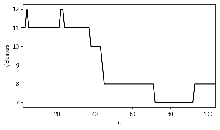
As we see here, increasing \(n_\mathrm{c}\) and therefore the density-threshold only yields less clusters which potentially means we are starting to loose information. To be sure, we can also double check the result with a somewhat larger radius to exclude that we already lost potential clusters with our first parameter combination.
[ ]:
r = 2
neighbourhoods, sort_order, revert_order = recipes.sorted_neighbourhoods_from_coordinates(langerin.input_data, r=r, sort_by="both")
langerin_neighbourhoods = cluster.Clustering(
    neighbourhoods, recipe="sorted_neighbourhoods"
)
[64]:
for c in tqdm(np.arange(0, 105, 1)):
    langerin_neighbourhoods.fit(radius_cutoff=r, similarity_cutoff=c, member_cutoff=10, v=False)
langerin.root._summary = langerin_neighbourhoods.root._summary
[65]:
df = langerin.summary.to_DataFrame()

c_values = df["similarity_cutoff"].to_numpy()
n_cluster_values = df["n_clusters"].to_numpy()

fig, ax = plt.subplots()
ax.plot(c_values, n_cluster_values, "k")
ax.set(**{
    "xlim": (c_values[0], c_values[-1]),
    "xlabel": "$c$",
    "ylabel": "#clusters",
    "yticks": range(np.min(n_cluster_values), np.max(n_cluster_values) + 1)
    })
[65]:
[(0.0, 104.0),
 Text(0.5, 0, '$c$'),
 Text(0, 0.5, '#clusters'),
 [<matplotlib.axis.YTick at 0x7fab186c0ca0>,
  <matplotlib.axis.YTick at 0x7fab19506910>,
  <matplotlib.axis.YTick at 0x7fab1a895d60>,
  <matplotlib.axis.YTick at 0x7fab186f4340>]]
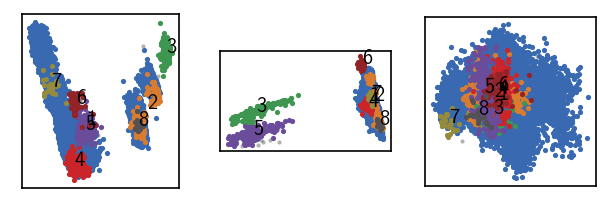
[47]:
langerin_neighbourhoods.fit(radius_cutoff=r, similarity_cutoff=1, member_cutoff=10)
langerin.labels = langerin_neighbourhoods.labels[revert_order]
draw_evaluate(langerin)
-----------------------------------------------------------------------------------------------
#points   r         nc        min       max       #clusters %largest  %noise    time
26528     2.000     1         10        None      8         0.962     0.001     00:00:0.691
-----------------------------------------------------------------------------------------------
[48]:
langerin_neighbourhoods.fit(radius_cutoff=r, similarity_cutoff=5, member_cutoff=10)
langerin.labels = langerin_neighbourhoods.labels[revert_order]
draw_evaluate(langerin)
-----------------------------------------------------------------------------------------------
#points   r         nc        min       max       #clusters %largest  %noise    time
26528     2.000     5         10        None      9         0.962     0.002     00:00:0.696
-----------------------------------------------------------------------------------------------
It looks like we obtain no additional cluster with the larger radius that is lost for the smaller one. For now we can deliberately stick with the smaller radius. We could now use manual hierarchical clustering to freeze the obtained clustering and increase the density-threshold only for a portion of the data set. Since this could become quite involved, though, we will not follow that route here and concentrate instead on the semi-automatic and automatic alternatives further below.
Semi-automatic hierarchical clustering
We described rationally guided, manual hierarchical clustering in the Hierarchical clustering basics tutorial using the isolate formalism. Here we want to take the different approach of generating a cluster hierarchy more or less automatically for a given cluster parameter range. We will use the radius of \(r=1.5\) from the last section and a grid of \(n_\mathrm{c}\) values to cluster subsequently with higher density-thresholds while we keep
track of the change in the cluster label assignments.
[7]:
r = 1.5
neighbourhoods, sort_order, revert_order = recipes.sorted_neighbourhoods_from_coordinates(langerin.input_data, r=r, sort_by="both")
langerin_neighbourhoods = cluster.Clustering(
    neighbourhoods, recipe="sorted_neighbourhoods"
)
We will start at \(n_\mathrm{c}=2\) but we will also need to determine a reasonable endpoint. To check the deduction of an upper bound from the number-of-neioghbours plot in the last section, let’s have a look at a clustering with a very high density-threshold.
[8]:
langerin_neighbourhoods.fit(radius_cutoff=r, similarity_cutoff=950)
langerin.labels = langerin_neighbourhoods.labels[revert_order]
draw_evaluate(langerin)
-----------------------------------------------------------------------------------------------
#points   r         nc        min       max       #clusters %largest  %noise    time
26528     1.500     950       None      None      4         0.314     0.430     00:00:3.710
-----------------------------------------------------------------------------------------------
At this point, the clustering seem to yield only clusters that are shrinking with even higher values for \(n_\mathrm{c}\). To perform a semi-automatic hierarchical clustering, we can use the HierarchicalFitter class HierarchicalFitterRepeat. This type uses a fitter repeatedly to build a cluster hierarchy.
[9]:
langerin_neighbourhoods._hierarchical_fitter = _fit.HierarchicalFitterRepeat(
    langerin_neighbourhoods.fitter
)
[10]:
# Make a range of c values with larger jumps towards the end
c_range = [2]
for _ in range(108):
    x = c_range[-1]
    c_range.append(max(x + 1, int(x * 1.05)))
print(c_range)
[2, 3, 4, 5, 6, 7, 8, 9, 10, 11, 12, 13, 14, 15, 16, 17, 18, 19, 20, 21, 22, 23, 24, 25, 26, 27, 28, 29, 30, 31, 32, 33, 34, 35, 36, 37, 38, 39, 40, 42, 44, 46, 48, 50, 52, 54, 56, 58, 60, 63, 66, 69, 72, 75, 78, 81, 85, 89, 93, 97, 101, 106, 111, 116, 121, 127, 133, 139, 145, 152, 159, 166, 174, 182, 191, 200, 210, 220, 231, 242, 254, 266, 279, 292, 306, 321, 337, 353, 370, 388, 407, 427, 448, 470, 493, 517, 542, 569, 597, 626, 657, 689, 723, 759, 796, 835, 876, 919, 964]
[11]:
langerin_neighbourhoods.fit_hierarchical(
    radius_cutoffs=r,
    similarity_cutoffs=c_range,
    member_cutoff=10
)
2025-04-11 11:46:54.557 | INFO     | __main__:<module>:1 - Running step 0     (r = 1.5, c = 2)
2025-04-11 11:46:54.873 | INFO     | __main__:<module>:1 - Running step 1     (r = 1.5, c = 3)
2025-04-11 11:46:55.188 | INFO     | __main__:<module>:1 - Running step 2     (r = 1.5, c = 4)
2025-04-11 11:46:55.504 | INFO     | __main__:<module>:1 - Running step 3     (r = 1.5, c = 5)
2025-04-11 11:46:55.824 | INFO     | __main__:<module>:1 - Running step 4     (r = 1.5, c = 6)
2025-04-11 11:46:56.140 | INFO     | __main__:<module>:1 - Running step 5     (r = 1.5, c = 7)
2025-04-11 11:46:56.460 | INFO     | __main__:<module>:1 - Running step 6     (r = 1.5, c = 8)
2025-04-11 11:46:56.782 | INFO     | __main__:<module>:1 - Running step 7     (r = 1.5, c = 9)
2025-04-11 11:46:57.102 | INFO     | __main__:<module>:1 - Running step 8     (r = 1.5, c = 10)
2025-04-11 11:46:57.423 | INFO     | __main__:<module>:1 - Running step 9     (r = 1.5, c = 11)
2025-04-11 11:46:57.745 | INFO     | __main__:<module>:1 - Running step 10    (r = 1.5, c = 12)
2025-04-11 11:46:58.068 | INFO     | __main__:<module>:1 - Running step 11    (r = 1.5, c = 13)
2025-04-11 11:46:58.395 | INFO     | __main__:<module>:1 - Running step 12    (r = 1.5, c = 14)
2025-04-11 11:46:58.723 | INFO     | __main__:<module>:1 - Running step 13    (r = 1.5, c = 15)
2025-04-11 11:46:59.049 | INFO     | __main__:<module>:1 - Running step 14    (r = 1.5, c = 16)
2025-04-11 11:46:59.377 | INFO     | __main__:<module>:1 - Running step 15    (r = 1.5, c = 17)
2025-04-11 11:46:59.709 | INFO     | __main__:<module>:1 - Running step 16    (r = 1.5, c = 18)
2025-04-11 11:47:00.037 | INFO     | __main__:<module>:1 - Running step 17    (r = 1.5, c = 19)
2025-04-11 11:47:00.367 | INFO     | __main__:<module>:1 - Running step 18    (r = 1.5, c = 20)
2025-04-11 11:47:00.696 | INFO     | __main__:<module>:1 - Running step 19    (r = 1.5, c = 21)
2025-04-11 11:47:01.026 | INFO     | __main__:<module>:1 - Running step 20    (r = 1.5, c = 22)
2025-04-11 11:47:01.354 | INFO     | __main__:<module>:1 - Running step 21    (r = 1.5, c = 23)
2025-04-11 11:47:01.683 | INFO     | __main__:<module>:1 - Running step 22    (r = 1.5, c = 24)
2025-04-11 11:47:02.016 | INFO     | __main__:<module>:1 - Running step 23    (r = 1.5, c = 25)
2025-04-11 11:47:02.349 | INFO     | __main__:<module>:1 - Running step 24    (r = 1.5, c = 26)
2025-04-11 11:47:02.678 | INFO     | __main__:<module>:1 - Running step 25    (r = 1.5, c = 27)
2025-04-11 11:47:03.010 | INFO     | __main__:<module>:1 - Running step 26    (r = 1.5, c = 28)
2025-04-11 11:47:03.343 | INFO     | __main__:<module>:1 - Running step 27    (r = 1.5, c = 29)
2025-04-11 11:47:03.677 | INFO     | __main__:<module>:1 - Running step 28    (r = 1.5, c = 30)
2025-04-11 11:47:04.014 | INFO     | __main__:<module>:1 - Running step 29    (r = 1.5, c = 31)
2025-04-11 11:47:04.350 | INFO     | __main__:<module>:1 - Running step 30    (r = 1.5, c = 32)
2025-04-11 11:47:04.682 | INFO     | __main__:<module>:1 - Running step 31    (r = 1.5, c = 33)
2025-04-11 11:47:05.016 | INFO     | __main__:<module>:1 - Running step 32    (r = 1.5, c = 34)
2025-04-11 11:47:05.352 | INFO     | __main__:<module>:1 - Running step 33    (r = 1.5, c = 35)
2025-04-11 11:47:05.690 | INFO     | __main__:<module>:1 - Running step 34    (r = 1.5, c = 36)
2025-04-11 11:47:06.030 | INFO     | __main__:<module>:1 - Running step 35    (r = 1.5, c = 37)
2025-04-11 11:47:06.372 | INFO     | __main__:<module>:1 - Running step 36    (r = 1.5, c = 38)
2025-04-11 11:47:06.710 | INFO     | __main__:<module>:1 - Running step 37    (r = 1.5, c = 39)
2025-04-11 11:47:07.051 | INFO     | __main__:<module>:1 - Running step 38    (r = 1.5, c = 40)
2025-04-11 11:47:07.388 | INFO     | __main__:<module>:1 - Running step 39    (r = 1.5, c = 42)
2025-04-11 11:47:07.919 | INFO     | __main__:<module>:1 - Running step 40    (r = 1.5, c = 44)
2025-04-11 11:47:08.536 | INFO     | __main__:<module>:1 - Running step 41    (r = 1.5, c = 46)
2025-04-11 11:47:09.074 | INFO     | __main__:<module>:1 - Running step 42    (r = 1.5, c = 48)
2025-04-11 11:47:09.543 | INFO     | __main__:<module>:1 - Running step 43    (r = 1.5, c = 50)
2025-04-11 11:47:10.020 | INFO     | __main__:<module>:1 - Running step 44    (r = 1.5, c = 52)
2025-04-11 11:47:10.463 | INFO     | __main__:<module>:1 - Running step 45    (r = 1.5, c = 54)
2025-04-11 11:47:10.864 | INFO     | __main__:<module>:1 - Running step 46    (r = 1.5, c = 56)
2025-04-11 11:47:11.294 | INFO     | __main__:<module>:1 - Running step 47    (r = 1.5, c = 58)
2025-04-11 11:47:11.645 | INFO     | __main__:<module>:1 - Running step 48    (r = 1.5, c = 60)
2025-04-11 11:47:12.002 | INFO     | __main__:<module>:1 - Running step 49    (r = 1.5, c = 63)
2025-04-11 11:47:12.356 | INFO     | __main__:<module>:1 - Running step 50    (r = 1.5, c = 66)
2025-04-11 11:47:12.715 | INFO     | __main__:<module>:1 - Running step 51    (r = 1.5, c = 69)
2025-04-11 11:47:13.077 | INFO     | __main__:<module>:1 - Running step 52    (r = 1.5, c = 72)
2025-04-11 11:47:13.438 | INFO     | __main__:<module>:1 - Running step 53    (r = 1.5, c = 75)
2025-04-11 11:47:13.804 | INFO     | __main__:<module>:1 - Running step 54    (r = 1.5, c = 78)
2025-04-11 11:47:14.175 | INFO     | __main__:<module>:1 - Running step 55    (r = 1.5, c = 81)
2025-04-11 11:47:14.547 | INFO     | __main__:<module>:1 - Running step 56    (r = 1.5, c = 85)
2025-04-11 11:47:14.925 | INFO     | __main__:<module>:1 - Running step 57    (r = 1.5, c = 89)
2025-04-11 11:47:15.306 | INFO     | __main__:<module>:1 - Running step 58    (r = 1.5, c = 93)
2025-04-11 11:47:15.692 | INFO     | __main__:<module>:1 - Running step 59    (r = 1.5, c = 97)
2025-04-11 11:47:16.084 | INFO     | __main__:<module>:1 - Running step 60    (r = 1.5, c = 101)
2025-04-11 11:47:16.479 | INFO     | __main__:<module>:1 - Running step 61    (r = 1.5, c = 106)
2025-04-11 11:47:16.876 | INFO     | __main__:<module>:1 - Running step 62    (r = 1.5, c = 111)
2025-04-11 11:47:17.282 | INFO     | __main__:<module>:1 - Running step 63    (r = 1.5, c = 116)
2025-04-11 11:47:17.696 | INFO     | __main__:<module>:1 - Running step 64    (r = 1.5, c = 121)
2025-04-11 11:47:18.117 | INFO     | __main__:<module>:1 - Running step 65    (r = 1.5, c = 127)
2025-04-11 11:47:18.544 | INFO     | __main__:<module>:1 - Running step 66    (r = 1.5, c = 133)
2025-04-11 11:47:18.977 | INFO     | __main__:<module>:1 - Running step 67    (r = 1.5, c = 139)
2025-04-11 11:47:19.419 | INFO     | __main__:<module>:1 - Running step 68    (r = 1.5, c = 145)
2025-04-11 11:47:19.874 | INFO     | __main__:<module>:1 - Running step 69    (r = 1.5, c = 152)
2025-04-11 11:47:20.342 | INFO     | __main__:<module>:1 - Running step 70    (r = 1.5, c = 159)
2025-04-11 11:47:20.831 | INFO     | __main__:<module>:1 - Running step 71    (r = 1.5, c = 166)
2025-04-11 11:47:21.332 | INFO     | __main__:<module>:1 - Running step 72    (r = 1.5, c = 174)
2025-04-11 11:47:21.846 | INFO     | __main__:<module>:1 - Running step 73    (r = 1.5, c = 182)
2025-04-11 11:47:22.378 | INFO     | __main__:<module>:1 - Running step 74    (r = 1.5, c = 191)
2025-04-11 11:47:22.917 | INFO     | __main__:<module>:1 - Running step 75    (r = 1.5, c = 200)
2025-04-11 11:47:23.486 | INFO     | __main__:<module>:1 - Running step 76    (r = 1.5, c = 210)
2025-04-11 11:47:24.064 | INFO     | __main__:<module>:1 - Running step 77    (r = 1.5, c = 220)
2025-04-11 11:47:24.662 | INFO     | __main__:<module>:1 - Running step 78    (r = 1.5, c = 231)
2025-04-11 11:47:25.292 | INFO     | __main__:<module>:1 - Running step 79    (r = 1.5, c = 242)
2025-04-11 11:47:25.933 | INFO     | __main__:<module>:1 - Running step 80    (r = 1.5, c = 254)
2025-04-11 11:47:26.593 | INFO     | __main__:<module>:1 - Running step 81    (r = 1.5, c = 266)
2025-04-11 11:47:27.279 | INFO     | __main__:<module>:1 - Running step 82    (r = 1.5, c = 279)
2025-04-11 11:47:27.976 | INFO     | __main__:<module>:1 - Running step 83    (r = 1.5, c = 292)
2025-04-11 11:47:28.718 | INFO     | __main__:<module>:1 - Running step 84    (r = 1.5, c = 306)
2025-04-11 11:47:29.496 | INFO     | __main__:<module>:1 - Running step 85    (r = 1.5, c = 321)
2025-04-11 11:47:30.328 | INFO     | __main__:<module>:1 - Running step 86    (r = 1.5, c = 337)
2025-04-11 11:47:31.194 | INFO     | __main__:<module>:1 - Running step 87    (r = 1.5, c = 353)
2025-04-11 11:47:32.110 | INFO     | __main__:<module>:1 - Running step 88    (r = 1.5, c = 370)
2025-04-11 11:47:33.089 | INFO     | __main__:<module>:1 - Running step 89    (r = 1.5, c = 388)
2025-04-11 11:47:34.116 | INFO     | __main__:<module>:1 - Running step 90    (r = 1.5, c = 407)
2025-04-11 11:47:35.163 | INFO     | __main__:<module>:1 - Running step 91    (r = 1.5, c = 427)
2025-04-11 11:47:36.268 | INFO     | __main__:<module>:1 - Running step 92    (r = 1.5, c = 448)
2025-04-11 11:47:37.407 | INFO     | __main__:<module>:1 - Running step 93    (r = 1.5, c = 470)
2025-04-11 11:47:38.582 | INFO     | __main__:<module>:1 - Running step 94    (r = 1.5, c = 493)
2025-04-11 11:47:39.887 | INFO     | __main__:<module>:1 - Running step 95    (r = 1.5, c = 517)
2025-04-11 11:47:41.256 | INFO     | __main__:<module>:1 - Running step 96    (r = 1.5, c = 542)
2025-04-11 11:47:42.768 | INFO     | __main__:<module>:1 - Running step 97    (r = 1.5, c = 569)
2025-04-11 11:47:44.457 | INFO     | __main__:<module>:1 - Running step 98    (r = 1.5, c = 597)
2025-04-11 11:47:46.274 | INFO     | __main__:<module>:1 - Running step 99    (r = 1.5, c = 626)
2025-04-11 11:47:48.271 | INFO     | __main__:<module>:1 - Running step 100   (r = 1.5, c = 657)
2025-04-11 11:47:50.563 | INFO     | __main__:<module>:1 - Running step 101   (r = 1.5, c = 689)
2025-04-11 11:47:52.891 | INFO     | __main__:<module>:1 - Running step 102   (r = 1.5, c = 723)
2025-04-11 11:47:55.202 | INFO     | __main__:<module>:1 - Running step 103   (r = 1.5, c = 759)
2025-04-11 11:47:57.685 | INFO     | __main__:<module>:1 - Running step 104   (r = 1.5, c = 796)
2025-04-11 11:48:00.350 | INFO     | __main__:<module>:1 - Running step 105   (r = 1.5, c = 835)
2025-04-11 11:48:03.124 | INFO     | __main__:<module>:1 - Running step 106   (r = 1.5, c = 876)
2025-04-11 11:48:06.250 | INFO     | __main__:<module>:1 - Running step 107   (r = 1.5, c = 919)
2025-04-11 11:48:09.602 | INFO     | __main__:<module>:1 - Running step 108   (r = 1.5, c = 964)
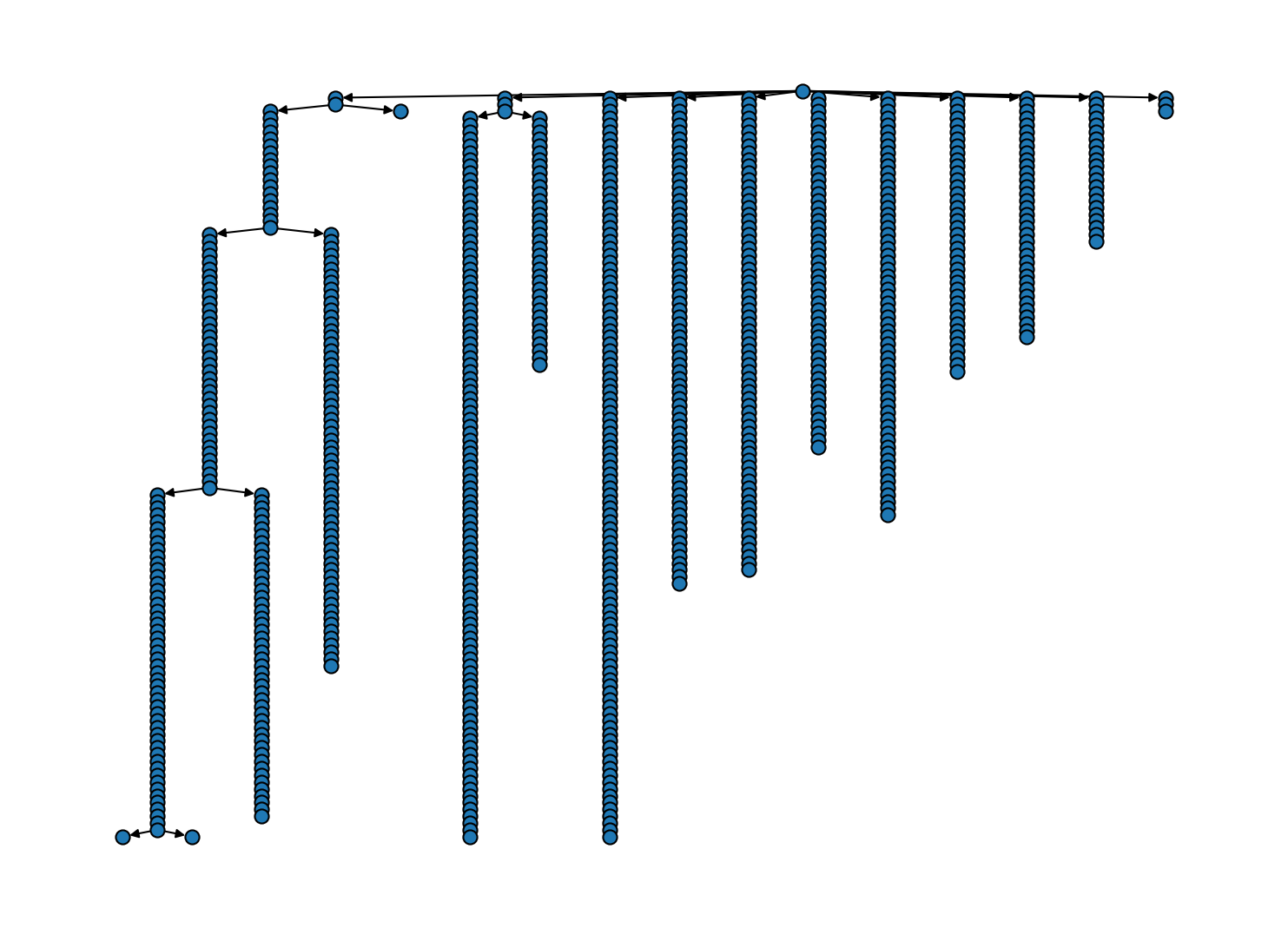
The resulting hierarchy of clusterings can be visualised either as a tree or pie plot.
[12]:
# Cluster hierarchy as tree diagram
#     (hierarchy level increasing from top to bottom)
fig, ax = plt.subplots(
    figsize=(
        mpl.rcParams["figure.figsize"][0] * 2.5,
        mpl.rcParams["figure.figsize"][1] * 3
    )
)
langerin_neighbourhoods.tree(
    ax=ax,
    draw_props={
        "node_size": 60,
        "node_shape": "o",
        "with_labels": False
    }
)

These diagrams can be admittedly hard to overlook because we have many hierarchy levels (one for each \(n_\mathrm{c}\) grid point). To reduces the cluster hierarchy to only a relevant number of bundles, we can apply some sort of trimming. A trimming protocol can be anything that traverses the bundle hierarchy (starting with the root bundle) and decides which bundles to keep, based on the bundle’s properties. We provide currently four basic trimming protocols: "trivial", "shrinking",
"lonechild", and "small". These can be triggered via Clustering.trim() under optional setting of the protocol keyword argument. Instead of a string to refer to a provided protocol, it is also possible to pass a callable that receives a bundle as the first argument and arbitrary keyword arguments.
The "trivial" protocol will remove the labels and all children on bundles that have all-zero cluster label assignments. The "shrinking" protocol removes the children on bundles that will never split again (only shrink). The "lonechild" protocol will replace a single child of a bundle with its grandchildren, and "small" removes bundles with less then member_cutoff members. Other protocols are conceivable and users are encouraged to implement their own.
Bundle processing is supported by the two generator functions _bundle.bfs and _bundles.bfs_leafs that allow to loop over bundles in a breadth-first-search fashion.
Let’s see what execution of the "trivial" protocol does to our tree. In fact, it is purely cosemetic in the present case because noise points are not used to create new bundles during the used hierarchical fitting.
[13]:
langerin_neighbourhoods['1.1.12'].labels
[13]:
array([0, 0, 0, 0, 0, 0, 0, 0, 0, 0])
[14]:
langerin_neighbourhoods['1.1.12'].children
[14]:
{}
[15]:
# Trim trivial nodes (has no effect here)
langerin_neighbourhoods.trim(langerin_neighbourhoods.root, protocol="trivial")
[16]:
# Cluster hierarchy as tree diagram
#     (hierarchy level increasing from top to bottom)
fig, ax = plt.subplots(
    figsize=(
        mpl.rcParams["figure.figsize"][0] * 2.5,
        mpl.rcParams["figure.figsize"][1] * 3
    )
)
langerin_neighbourhoods.tree(
    ax=ax,
    draw_props={
        "node_size": 60,
        "node_shape": "o",
        "with_labels": False
    }
)
[17]:
langerin_neighbourhoods['1.1.12'].labels
[18]:
langerin_neighbourhoods['1.1.12'].children
[18]:
{}
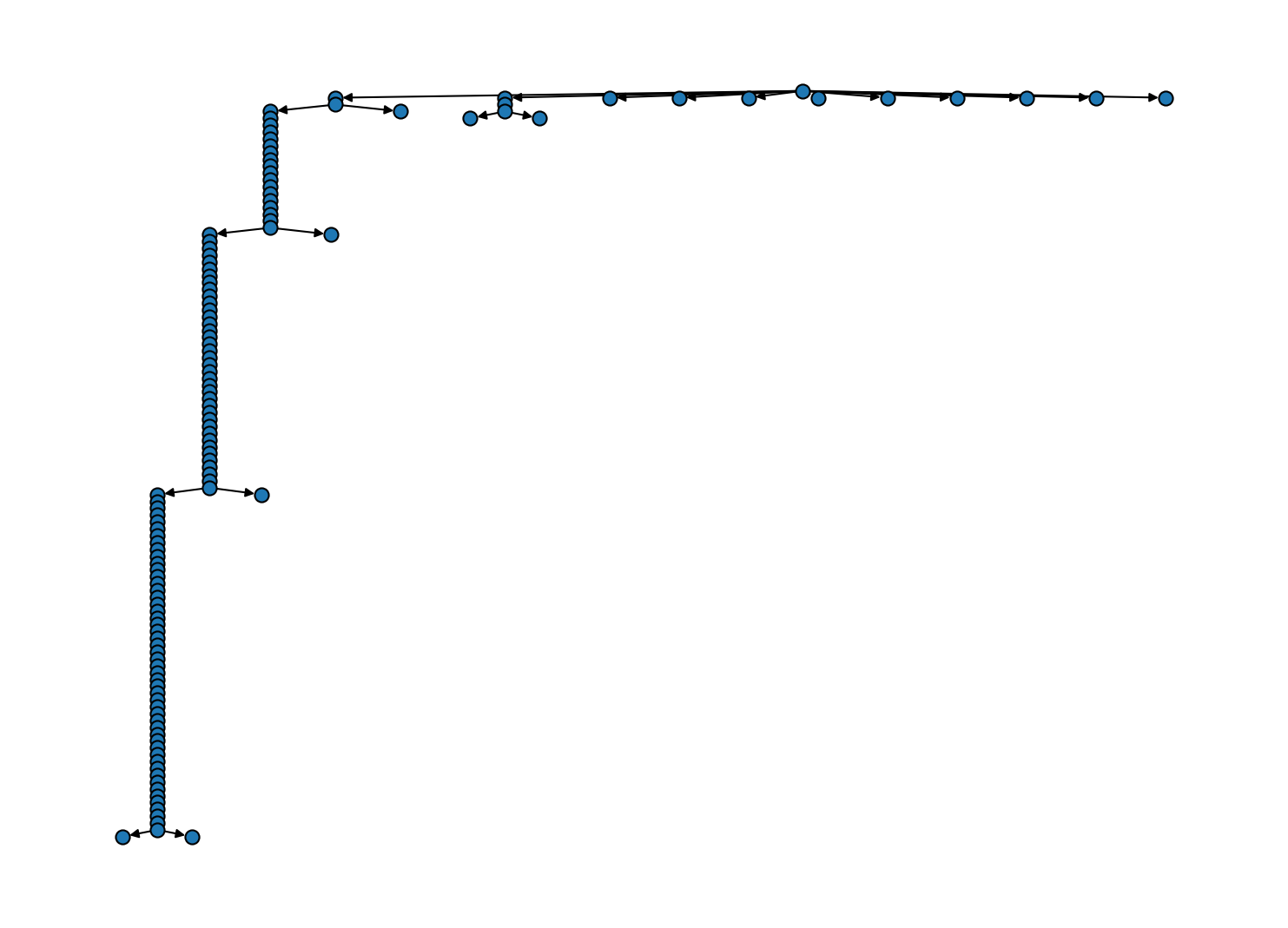
The "shrinking" protocol on the other hand has a major effect. Of all the bundles in the tree above, we will keep only those that emerge from an immediate split into sub-clusters. Bundles created as the sole child of a parent will be removed if there is no further split further down the line. Note that this will still keep lone children if there is an actual split downstream.
[19]:
# The "shrinking" protocol is the default
langerin_neighbourhoods.trim(langerin_neighbourhoods.root)
[20]:
# Cluster hierarchy as tree diagram
#     (hierarchy level increasing from top to bottom)
fig, ax = plt.subplots(
    figsize=(
        mpl.rcParams["figure.figsize"][0] * 2.5,
        mpl.rcParams["figure.figsize"][1] * 3
    )
)
langerin_neighbourhoods.tree(
    ax=ax,
    draw_props={
        "node_size": 60,
        "node_shape": "o",
        "with_labels": False
    }
)
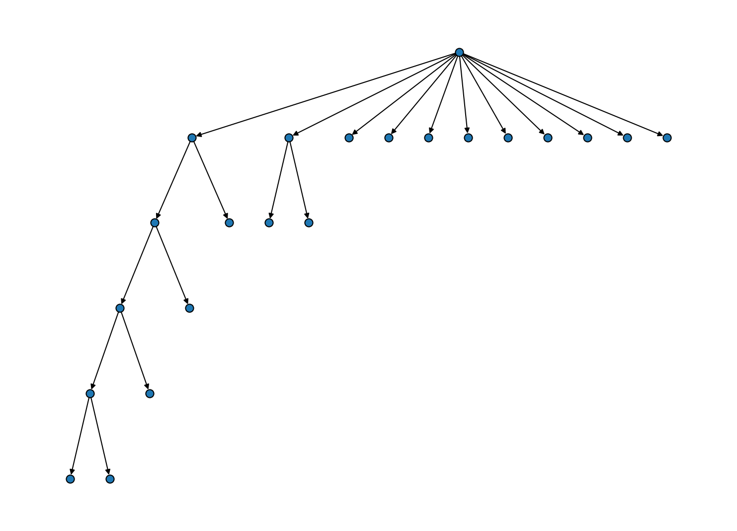
Another simplification is achieved through the "lonechild" protocol that will remove all the intermediate sole bundles at hierarchy levels where a cluster is only shrinking.
[21]:
# Remove levels on which only one child appears
langerin_neighbourhoods.trim(langerin_neighbourhoods.root, protocol="lonechild")
[22]:
# Cluster hierarchy as tree diagram
#     (hierarchy level increasing from top to bottom)
fig, ax = plt.subplots(
    figsize=(
        mpl.rcParams["figure.figsize"][0] * 2.5,
        mpl.rcParams["figure.figsize"][1] * 2
    )
)
langerin_neighbourhoods.tree(
    ax=ax,
    draw_props={
        "node_size": 60,
        "node_shape": "o",
        "with_labels": False
    }
)
And we can finally put everything together and incorporate the child clusters into the root data set. Note that for this, the "shrinking" protocol would have been sufficient.
[23]:
langerin_neighbourhoods.reel()
After this call, cluster labeling may not be contiguous and sorted by size, which we can fix easily, though.
[24]:
langerin_neighbourhoods.root._labels.sort_by_size()
[ ]:
langerin.labels = langerin_neighbourhoods.labels[revert_order]
draw_evaluate(langerin)
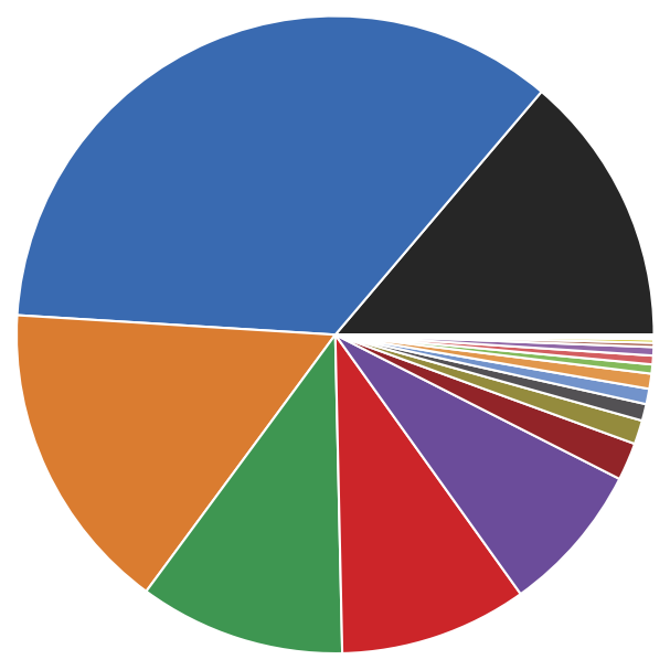
[27]:
# Cluster hierarchy as pie diagram
#     (hierarchy level increasing from the center outwards)
_ = langerin.pie(
    pie_props={"normalize": True}
)
plt.xlim((-0.3, 0.3))
plt.ylim((-0.3, 0.3))
[27]:
(-0.3, 0.3)
[36]:
print("Label Size")
print("==========")
print(*(f"{l:>5} {s:>4}" for l, s in sorted({k: len(v) for k, v in langerin.root._labels.mapping.items()}.items())), sep="\n")
Label Size
==========
    0 3661
    1 9344
    2 4210
    3 2774
    4 2528
    5 2029
    6  507
    7  322
    8  225
    9  207
   10  203
   11  123
   12  118
   13  113
   14   57
   15   46
   16   26
   17   16
   18   10
   19    9
For later re-use, we can remember the clustering parameters leading to the isolation of each cluster and save the cluster labels.
[37]:
np.save("md_example/langerin_labels.npy", langerin.labels)
[38]:
print("Label", "r", "n", sep="\t")
print("-" * 20)
for k, v in sorted(langerin_neighbourhoods.root._labels.meta["params"].items()):
    print(k, *v, sep="\t")
Label   r       n
--------------------
1       1.5     964
2       1.5     5
3       1.5     964
4       1.5     2
5       1.5     93
6       1.5     22
8       1.5     2
9       1.5     2
10      1.5     2
12      1.5     2
13      1.5     2
14      1.5     5
15      1.5     2
16      1.5     2
17      1.5     2
19      1.5     4
Automatic hierarchical clustering
Semi-automatic clustering as demonstrated in the last section works reasonably well in our example. The need to screen potentially a lot of parameter combinations, however, to build a hierarchy from threshold-based slices can be seen as fundamentally flawed. We also offer a more rigorous directly hierarchical clustering procedure as an alternative. This fully hiearchical clustering outperforms semi-automatic clustering in several aspects:
We only need to specify a neighbour search radius r
We can be sure that we won’t miss relevant threshold values, i.e.
all splits will be seen in the hierarchy
clusters as obtained will have their maximum possible extend
[ ]:
# Select a fast clustering recipe
r = 1.5
neighbourhoods, sort_order, revert_order = recipes.sorted_neighbourhoods_from_coordinates(langerin.input_data, r=r, sort_by="both")
langerin_neighbourhoods = cluster.Clustering(
    neighbourhoods, recipe="sorted_neighbourhoods_mst"
)
[41]:
langerin_neighbourhoods.fit_hierarchical(radius_cutoff=r, member_cutoff=10)
2025-04-11 12:00:29.918 | INFO     | __main__:<module>:1 - Started hierarchical CommonNN clustering - HierarchicalFitterExtCommonNNMSTPrim
2025-04-11 12:07:20.216 | INFO     | commonnn.report:wrapper:248 - Built MST
2025-04-11 12:07:20.275 | INFO     | __main__:<module>:1 - Computed Scipy Z matrix
2025-04-11 12:07:21.435 | INFO     | __main__:<module>:1 - Built bundle hierarchy from Scipy Z matrix
2025-04-11 12:07:21.445 | INFO     | __main__:<module>:1 - Converted all leafs to root labels
The present implementation is still experimental. It currently includes by default the construction of a Scipy compatible Z-matrix, which represents a binary tree of bottom-up merges of data points or clusters at decreasing density thresholds:
[ ]:
# Cluster a, cluster b, density threshold, member count
langerin_neighbourhoods._hierarchical_fitter._artifacts["Z"]
array([[0.0000e+00, 3.0000e+00, 5.3240e+03, 2.0000e+00],
       [2.0000e+00, 5.0000e+00, 5.2230e+03, 2.0000e+00],
       [1.4000e+01, 2.6529e+04, 5.1540e+03, 3.0000e+00],
       ...,
       [2.6483e+04, 5.3051e+04, 0.0000e+00, 2.6526e+04],
       [2.6482e+04, 5.3052e+04, 0.0000e+00, 2.6527e+04],
       [2.6481e+04, 5.3053e+04, 0.0000e+00, 2.6528e+04]])
From this, a hierarchy of Bundle instances is created in a second step. Here we already apply a member_cutoff to decide when a split results in two relevant clusters or just represents the shrinking of a parent cluster. In this step, lone child nodes will be already removed as well. Furthermore we resolve binary structure of the tree so that a parent can have more than two children if they arise from a split at the same density threshold. So to some extend, this includes a processing of
the hierarchy as shown for the semi-automatic case already. Both the Scipy and bundle hierarchy building step can be suppressed with scipy_hierarchy=False and bundle_hierarchy=False.
It should be noted that for technical reasons the bundles do not carry labels yet, but collect their members in a bundle.graph object (currenly just a Python set). If make_labels=True (default) the leaf nodes of the bundle hierarchy will be used to set labels on the root bundle, though, in the end.
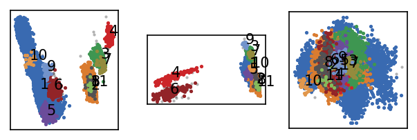
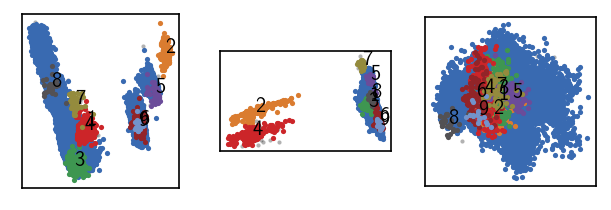
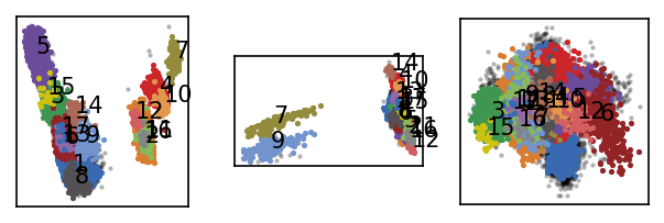
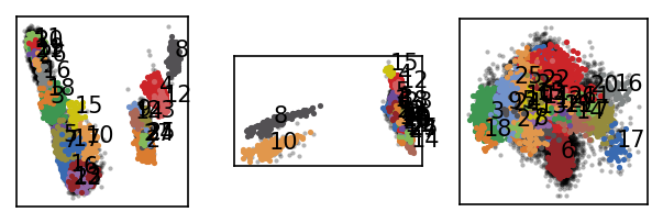
[44]:
langerin.labels = langerin_neighbourhoods.labels[revert_order]
langerin.root._labels.sort_by_size()
draw_evaluate(langerin)
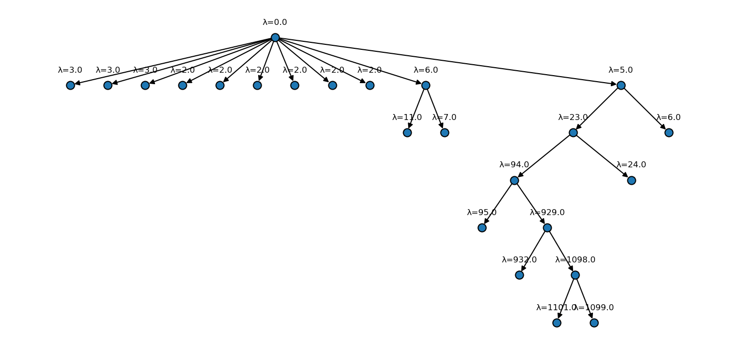
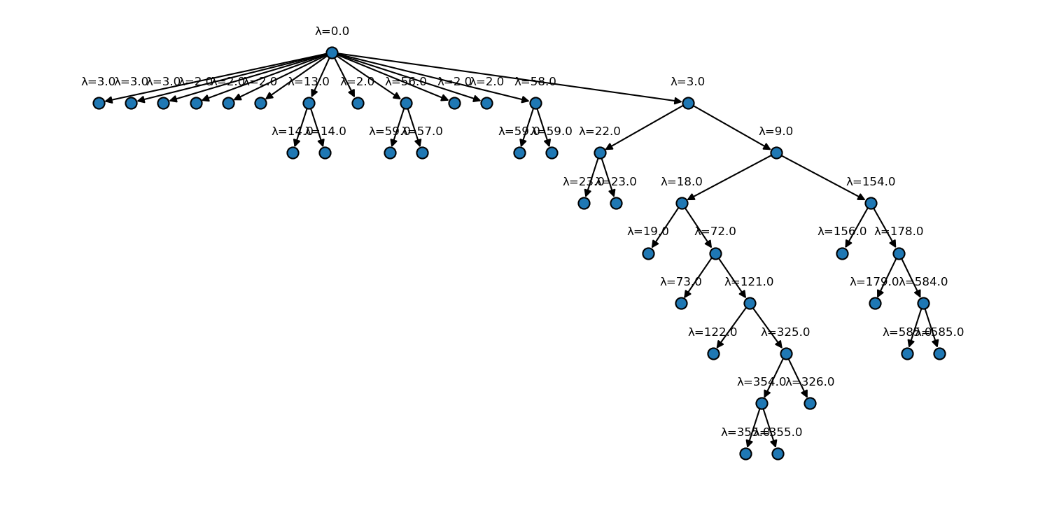
[51]:
fig, ax = plt.subplots(
    figsize=(
        mpl.rcParams["figure.figsize"][0] * 2.5,
        mpl.rcParams["figure.figsize"][1] * 2
    )
)
langerin_neighbourhoods.tree(
    ax=ax,
    draw_props={
        "node_size": 60,
        "node_shape": "o",
        "with_labels": False
    },
    annotate=True,
    annotate_format="λ={lambda}"
)
[45]:
print("Label Size")
print("==========")
print(*(f"{l:>5} {s:>4}" for l, s in sorted({k: len(v) for k, v in langerin.root._labels.mapping.items()}.items())), sep="\n")
Label Size
==========
    0 5715
    1 7606
    2 4210
    3 2795
    4 2532
    5 2049
    6  523
    7  228
    8  214
    9  208
   10  119
   11  114
   12   57
   13   53
   14   48
   15   29
   16   18
   17   10
The clustering result is largely equivalent to what we obtained in the semi-automatic run before with the difference that this time the clusters are not taken from arbitrary slices of the hierarchy. A semi-automatic clustering would need to use an increment of 1 in \(n_\mathrm{c}\) over the full parameter range to reach the same accuracy. We can also note that the current hierarchy yields an additional split far down at \(n_\mathrm{c}=1098\), a value that we did not include in the semi-automatic parameter range. Before this background, it seems acceptable that the fully hierarchical clustering is by a factor of 5 times slower in this direct comparison (6:51 vs. 1:20 minutes).
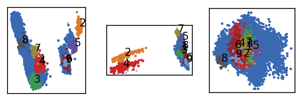
Let’s finish here with a another look at the choice of the neighbourhood radius r. Since the fully hierarchical approach allows us to play with this parameter without worrying about changing similarity threshold values, it is easy to compare full hierarchies side by side. At smaller radii, the clustering can become orders of maginitude faster. Ideally, the end result is not very sensisitive to the actual choice of r at all. At smaller and smaller radii, however, we may cross over from having a representative local density estimate that resolves all density differences nicely to a noisy estimate that creates artifical splits. Below we see additional clusters emerging for a lower radius. Whether this still makes sense, has to be validated in context.
[56]:
# Select a fast clustering recipe
r = 1.2
neighbourhoods, sort_order, revert_order = recipes.sorted_neighbourhoods_from_coordinates(langerin.input_data, r=r, sort_by="both")
langerin_neighbourhoods = cluster.Clustering(
    neighbourhoods, recipe="sorted_neighbourhoods_mst"
)
[57]:
langerin_neighbourhoods.fit_hierarchical(radius_cutoff=r, member_cutoff=10)
2025-04-11 12:54:40.331 | INFO     | __main__:<module>:1 - Started hierarchical CommonNN clustering - HierarchicalFitterExtCommonNNMSTPrim
2025-04-11 12:56:03.711 | INFO     | commonnn.report:wrapper:248 - Built MST
2025-04-11 12:56:03.764 | INFO     | __main__:<module>:1 - Computed Scipy Z matrix
2025-04-11 12:56:05.021 | INFO     | __main__:<module>:1 - Built bundle hierarchy from Scipy Z matrix
2025-04-11 12:56:05.029 | INFO     | __main__:<module>:1 - Converted all leafs to root labels
[58]:
langerin.labels = langerin_neighbourhoods.labels[revert_order]
langerin.root._labels.sort_by_size()
draw_evaluate(langerin)
[59]:
fig, ax = plt.subplots(
    figsize=(
        mpl.rcParams["figure.figsize"][0] * 2.5,
        mpl.rcParams["figure.figsize"][1] * 2
    )
)
langerin_neighbourhoods.tree(
    ax=ax,
    draw_props={
        "node_size": 60,
        "node_shape": "o",
        "with_labels": False
    },
    annotate=True,
    annotate_format="λ={lambda}"
)
[60]:
print("Label Size")
print("==========")
print(*(f"{l:>5} {s:>4}" for l, s in sorted({k: len(v) for k, v in langerin.root._labels.mapping.items()}.items())), sep="\n")
Label Size
==========
    0 10596
    1 4644
    2 3238
    3 2851
    4 2522
    5  707
    6  384
    7  294
    8  225
    9  188
   10  185
   11  162
   12  119
   13   87
   14   57
   15   46
   16   40
   17   37
   18   26
   19   24
   20   17
   21   13
   22   13
   23   12
   24   11
   25   10
   26   10
   27   10